- Table of contents
- Workflow Overview
- CODE ORGANIZATION AND DESIGN
Workflow Overview
WORKFLOW FOR THE PRODUCTION OF ENVIRONMENTAL CLIMATE LAYERS
NCEAS-IPLANT-NASA
Benoit Parmentier, July 1, 2013
Project’s goal
The goal of the project is to produce three primary daily climate products pertaining to: maximum temperature, minimum temperature and precipitation. Products will cover the world (with the exception of Antarctica) at a one kilometer resolution for the 1970-2010 time period.
Introduction
This document sketches a tentative workflow for the production of climate environmental layers. It is a first attempt at outlining the various stages and challenges that will be encountered during the production of the global climate layers.

The first section presents the general logic and organization for the current workflow while the second section provides specific details on the implementation of steps in R and Python languages.
- GENERAL LOGIC AND ORGANIZATION
We have broadly defined three stages in the workflow: data preparation, interpolation and assessment.
STAGE 1: DATA PREPARATION
This stage corresponds to the preparation of the datasets for input in the interpolation stage. Datasets can be prepared for any study area or regions but corresponding matching MODIS tiles must be provided or queried.
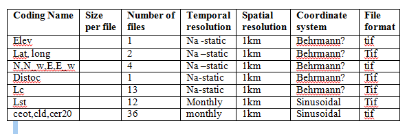
Raster covariate data production
Raster layers from various inputs must be derived before the interpolation. This step includes downloading, processing and derivation of covariates at a one kilometer scale.
LST climatology averages are produced following screening of values based on Quality flags for MOD11A1 version 5. Averages are calculated over 10 years (2001-2010) for each month for both day and night. Monthly averages for the day are used in maximum air temperature interpolation while monthly averages for the night are used in minimum air temperature interpolation.
Table of covariates

Challenges and Issues
- Should we produce all covariates at the global scale or produce them on the fly for each processing tile/region during the interpolation stage? (current approach)
- Which projection should be used to store global layers for intermediary processes (Behrmann?)
- Will covariate layers also be served as additional end products? For instance the clouds products fused SRTM, Land Cover Consensus data or LST climatology may be of great interest to ecologists and other scientists.
Current codes
Specifications and estimated size of inputs
TBD
Specifications and estimated size of outputs
TBD
Station Database production
This step includes downloading of station datasets from the internet and from other storage devices such as DVD. The process will include the organization or reorganization of datasets in tables to allow querying based on time (daily and monthly time step), station ID and location. GHCN is expected to be the most important source but additional datasets (such as the FAO climatologies) will be included. Since some data source may contain monthly information only, the project will necessitate the creation of monthly and daily databases (to be decided/discussed). Data sources are of different quality therefore it will be necessary to retain the quality information for all input datasets. Since the GHCN database has undergone a very stringent quality process, it is probably the most reliable source. We can potentially follow the approach described in Hijmans et al. 2005 and use stations from lesser known sources only in cases there are insufficient numbers of stations drawn from the GHCN.
Queries can be made over different time period (i.e. 1980-2011 or 200-2011) and the current codes allow for varying the time period of the queries. Options are also provided to take into account GHCND flags values.
Challenges and Issues
- Should we use one or multiple database at the daily and monthly time scale?
- How do we deal with the multiple quality and redundancy from sources?
- Will some quality procedures be put in place to assess the quality of input data?
- How often will the station database be updated?
- Will the covariate information be included in the database or extracted tile by tile during the interpolation process?
Current codes
- Station database production code:
download-ghcn-daily.sh
ghcn-to-psql.R" - Station Data preparation code:
Database_stations_covariates_processing_function.R
Specifications and estimated size of inputs
TBD
Specifications and estimated size of outputs
TBD
STAGE 2: INTERPOLATION*
Model fitting
Interpolation is done by processing the globe tile by tile and fitting models for each tile/region. Before fitting, the database is queried to obtain the design matrix for all stations within the current processing tile and within a given buffer distance. A buffer is used to include neighboring stations outside the tile in order to minimize the edge effects and provide zones of overlaps contiguous predictions (this is currently being added to the code). In some cases, the number of stations in specific processing tiles is insufficient to fit models so we will need to either expand further the buffer “on-the-fly” to query additional areas around the processing tile or provide some pre-planned processing/fitting regions. At this stage, it is assumed that station data includes covariates so that it is not necessary to load raster images in memory during the model fitting. Note that at this stage, both monthly and daily model fitting must be performed. Fitting and validation stations must be clearly labeled and tracked throughout the fitting and prediction steps. Fitting is done in a local projection system that minimizes distortions in shape and distances (currently using Lambert Conic Conformal). Methods currently implemented include: GAM CAI, GAM fusion, GAM_daily, Kriging_daily, and GWR_daily. Workflow must include a backup algorithm to account for problems in running some methods of interpolation.
Before fitting, meteorological stations are divided randomly into training and validation datasets. The proportion retained for sampling may be varied within a range of values and multiple numbers of samples may be drawn for specific hold out proportion (default holdout proportion is 30%). Also provided is an option to retain the same training sample for every day of the year. Additional sampling scheme may be added at later times.
Challenges and Issues
- Should model fitting be kept separate from prediction steps by retaining covariates information in the database?
- Hold out is currently done at the daily time scale. Should hold-out be carried out at the monthly time scale for multiple scale methods?
- How can the sampling strategy best estimate the effect of lack of data and autocorrelation present in both the validation and training samples?
- How advanced and specific should the sampling strategy be given that this is a global application?
Current codes
- GAM fusion and GAM CAI fitting:
GAM_fusion_function_multisampling.R - Sampling:
sampling_script_functions.R
Model Prediction
During prediction, raster covariate images overlapping the current tile being processed are loaded and values are predicted for every pixel at one kilometer resolution. Predictions must be done in the local projection system used in fitting and may require reprojection of the raster covariate layers on the fly. This step is potentially slow and is currently parallelized. In multi time scale methods, both monthly and daily predictions must be carried out to obtain a final prediction. This process of prediction is the most time intensive part of the workflow.
Challenges and Issues
- How are projections and reprojections going to be handled? This step must be minimized because it is time consuming and will impact the workflow.
- Which projection should be used? A possibility is to use a Lambert Conformal Conic with 2 standard parallels and one central meridian. The location of the meridian and parallels can be adjusted on the fly depending on the size of the processing area/tile. We can also modify the choice of projection depending on the shape of the processing region and its latitude.
- What tiling system should be used? MODIS tiles suffer from extreme shape alterations in the middle and higher latitudes. We may need to organize processing regions using a different tiling system based on a new projection.
- What will be the file format used for the intermediate steps? A multiband file such as NCDF may be useful to store model parameters, fitting stations and other metadata information during processing. Currently all information is saved in tif and RData files.
- Will uncertainty at each pixel be generated during the prediction stage? This will affect both the size of outputs and time of production. Furthermore, in the case of multiple time scale methods, we will need to derive some method to compute uncertainty from monthly to daily predictions.
Current codes
- Design matrix extraction:Database_stations_covariates_processing_function.R
- Gam_fusion, gam_CAI: GAM_fusion_function_multisampling.R
- GAM_daily, Kriging_daily, GWR_daily: interpolation_method_day_function_multisampling.R
- Raster prediction: GAM_fusion_analysis_raster_prediction_multisampling.R
Specifications and estimated size of inputs
TBD
Specifications and estimated size of outputs
TBD
STAGE 3: ASSESSMENT AND VALIDATION
Validation is performed using testing stations and various metrics such as MAE, RMSE and Pearson R correlation. At this stage, individual maps and diagnostic plots (i.e. predicted versus observed) are automatically produced for any given dates. Monthly averages for accuracy metrics are also computed to evaluate the effect of season on the accuracy of predictions. Covariates and input meteorological station data are also assessed through reports on statistics and figures. At a later stage, this stage may include a quality check of the predictions to flag errors and to assess the final product.
Challenges and Issues
- Will a pixel quality information layer be included in the final product (in addition to uncertainty)?
- Will accuracy in term of distance to closest fitting station be supplied? This may useful information.
Current codes
- GAM_fusion_function_multisampling_validation_metrics.R
- results_covariates_database_stations_output_analyses.R
- results_interpolation_date_output_analyses.R
Estimated size of inputs
TBD
Estimated size of outputs
TBD
CODE ORGANIZATION AND DESIGN
The code is organized in 14 source files. There are 12 source files written in R and 2 source files written in python. Interpolation can be run by setting parameters and arguments in one unique script: the master script. All remaining source files contain functions that perform individual tasks related to the downloading, processing, interpolation and accuracy assessment. The code is highly extensible. For instance, additional sampling scheme or methods may be added with a few targeted changes. In the future, the master script may be modified to run interpolation as a shell command. The code is organized in five “stages” with* possibility of running *each stage separately by providing a list of parameters.
Description of Processing Stages
STAGE 1: LST processing
downloading of MODIS tiles and calculation of climatology/averages.
STAGE 2: Covariates preparation
production of covariates for interpolation, this includes cropping, reprojection, calculation of aspect, distance to coast for a specific processing region.
STAGE 3: Data preparation
a subset of meteorological stations used in the interpolation is created by database query and extraction of covariates.
STAGE 4: Raster prediction
creation of testing and training samples, fitting of models and prediction for a given region and method (i.e. gam fusion, Kriging). This step also includes the calculation of validation metrics.
STAGE 5: Output analyses
visualization of results for specific dates and plots of predicted versus observed values.
Table of source files
| Stage | Purpose | Source File |
|---|---|---|
| - | Set parameters for interpolation and perform predictions | master_script_temp.R |
| 1 | Modis download | LST_modis_downloading.py |
| 1 | LST climatology python script | LST_climatology.py |
| 1 | Set environment for GRASS use in shell | grass-setup.R |
| 1 | Tile processing, climatology and downloading | download_and_produce_MODIS_LST_climatology.R |
| 2 | Covariate preparation | covariates_production_temperatures.R |
| 3 | Database query and covariate extraction | Database_stations_covariates_processing_function.R |
| 4 | Sampling Scheme | sampling_script_functions.R |
| 4 | Multiple time scale interpolation methods | GAM_fusion_function_multisampling.R |
| 4 | Single time scale interpolation methods | interpolation_method_day_function_multisampling.R |
| 4 | Interpolation, main script calling functions for sampling and fitting | GAM_fusion_analysis_raster_prediction_multisampling.R |
| 4 | accuracy metric calculation | GAM_fusion_function_multisampling_validation_metrics.R |
| 5 | Results assessment plots | results_interpolation_date_output_analyses.R |
| 5 | covariates analyses | results_covariates_database_stations_output_analyses.R |
Additional information on function and their parameters will be provided in additional tables.
MASTER SCRIPT PARAMETERS AND ARGUMENTS
Main parameters used for temperature predictions
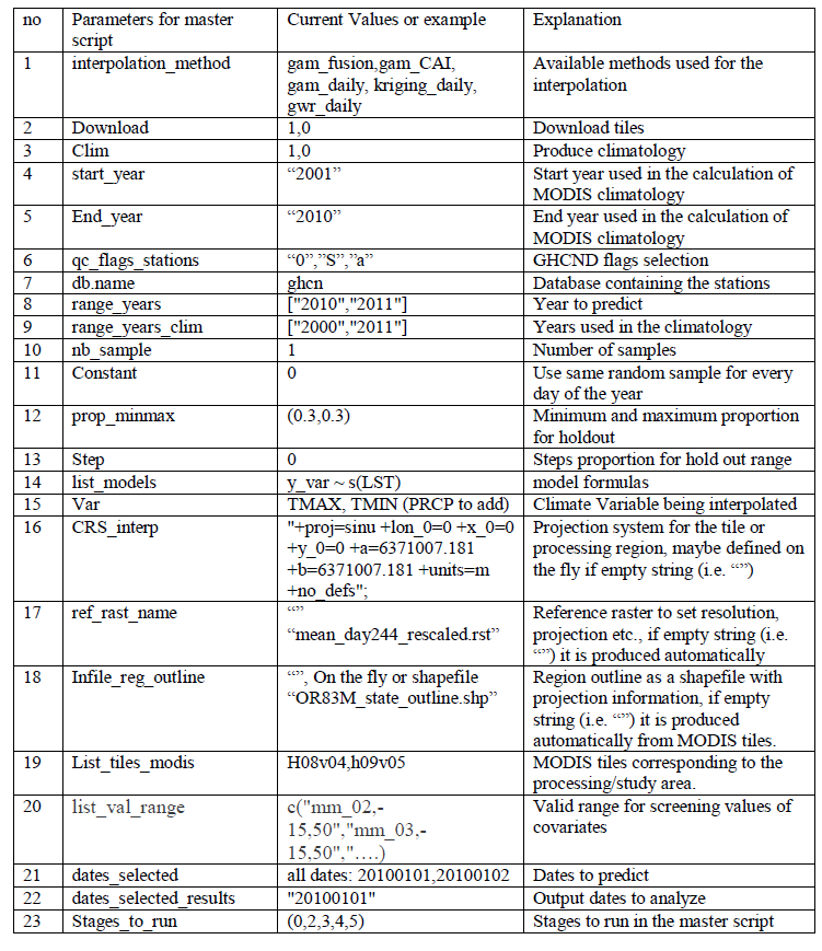
Note that there are many more parameters necessary to allow the prediction to run. These are included in the following table.
Additional parameters used to set inputs and outputs

Parallelization: Potential issues to resolve
A major question remains concerning parallelization of processes: “How can the number of cores be adjusted for processing regions in terms of availability of memory?
Many functions in the scripts are designed to be run using “mclapply” from the package parallel. Experimentation using the Venezuela, Oregon and Queensland regions shows that the number of cores must be adjusted to account for memory usage. This is particularly challenging since regions may vary in size as well as in terms of the number of valid pixels. For instance, the Oregon region covers about half a MODIS tile while Venezuela and Queensland regions cover 6 MODIS tiles (2400x3600). For Oregon, many functions can be run with 12 cores on Atlas while this number must be reduced to 9 or 6 for Venezuela. Furthermore, since Queensland contains more land area (and less NA) and has more fitted models, the number of cores must be adjusted to take into account the memory usage while prediction in raster format takes place.